|
|
|

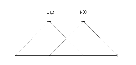
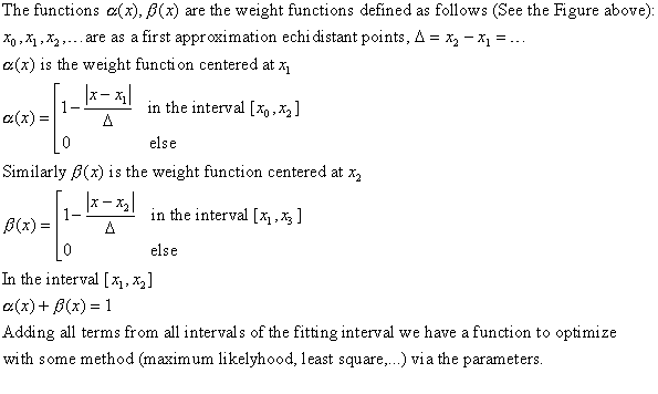
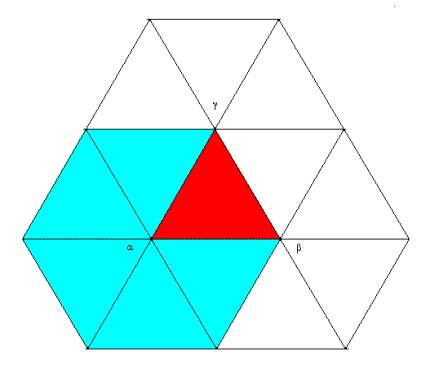
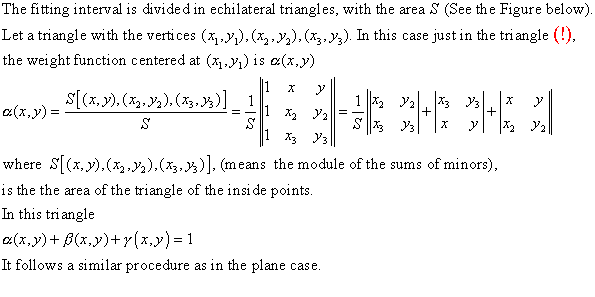
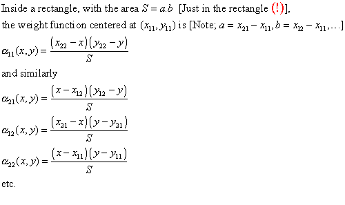
What is (I suppose) new, the empirical function, which one is a superposition
of some functions, non continues in derivatives, not easy to calculate by hand,
but easy for a computer.



An example in the small, old program [plane_1.ZIP],
[data.ZIP], [RLZRUN20.ZIP],
containing a lot of bugs, can be used to test the method. Extract in a directory and install.
Starting the program we see two small form windows.
In the window "MainR1", we can choose between two ways of introducing the input data.
Pressing the "DateKEYB" button, it appears a spreadsheet where we
can insert a set of data.
The spreadsheet input is a number of rows of XM, YM, ZM triplets, the
experimental data. Selecting one by one the cells of a row, by a click,
introducing the corresponding values and validating the row by an ENTER, we can
fill this input. Actually they are necessary at least of NM = 9 input points.
The program automatically updates the NM and the XMIN, XMAX, YMIN, YMAX, ZMIN,
ZMAX (the minimum minimorum and the maximum maximorum of input x, y, z) values,
necessary later.
From this point the procedure is the same as for the second way.
The second way begins with a click on the dropdown combo, which one presents
a lot of files with different input and output data.
Corresponding, they are two kinds of files in the dropdown combo.
The ???????i.dat and the ???????c.dat files. The "i" files contains
just the different input data, the "c" files the input and the
calculated values (the precision indices of the fit, the parameters of the
empirical functions...).
From the dropdown combo we can choose a file with some test data and with a
click on DateDISK start the procedure.
Again appears the spreadsheet, now with the data from the selected data file.
The format of the input file is, line by line:
A line with
XMIN, XMAX, NX, NVX #####.##, #####.##,
##, ##
where NX-1 is the number of subintervals on the x axis
and NXV the "node-sections" on the x axis
(actually don't work)
similar a line for the y values:
YMIN, YMAX, NY, NVY #####.##, #####.##,
##, ##
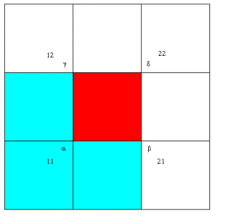
The NX*NY points divides in (NX-1)*(NY-1) rectangles the
xy-plane.
The next line contains the number of input,
"experimental", values
NM ####
followed by the triplets, NM times*3 lines
XM #####.##
YM #####.##
ZM #####.##
A click on the "Retea" button, followed by a click on the
"Mcmmp" button, some patience, and we can see the results, mainly in
the second forms window, "Log 2".
In this window appears the precision indices:
OMEGA=[sum of (ZM-ZC)**2 over NM] / ( NM- 9 )
where ZC are by the empirical function calculated values
with the following remark:
IF (NM-9)=0 THEN
OMEGA=999
PZO=999
ELSE
PZO= 0.6745*SQRT( OMEGA)
The chi-square value is calculated as:
HI=sum of (ZM-ZC)**2 / ZC over NM
Remark:
- we can edit the input data of any &quoot;i" file
- we can use the "o" files as input files
At the other hand, we can use the spreadsheet window to calculate some
particular values, introducing X, Y and then clicking in Z for the calculated
value.
If we want, we can see the results graphically, clicking on the "GraficR"
button from the spreadsheets window.
The red bars are the z-distances of the input values up from the calculated
surface values, the blue are the same for that input values "under"
the surface. The black lines sketch’s the empirical surface. The buttons
"JOS", "STANDARD", "SUS" makes visible/invisible
the red, black and blue points. For better visibility the figure can be rotated
by left or right clicks on the buttons "RotireY" and
"RotireZ", around the fictive y and z axis.
Attention! On the first click on the "Grafic" window reappears the
"MainR" window where we can save the calculated data. With a new
click in the graphics window we can continue the inspection.
After saving the output data, we can start again with new data in the
"MainR" window.
Attention! Please don't close the "old" spreadsheet (Tabela x) and
graphics (Grafic xxx) windows, here is a bug. In that time, in a schizophrenic
tentative, I have tried to develop my "big" method" and to learn
the CA Realizer 2, simultaneously.
To do (as I have learned from the Linux fans):
- to compare the method with other simillar methods, concerning the speed, the
efficiency (precision/number of parameters)
- to generalize for different divisions in rectangles and, why not, triangles,
or other plane figures
- to generalize for other dimensions
>
- to introduce the eventually known resttrictions, slops etc.
- to replace my simplest least-square fiit with other, sophisticated one,
maximum likelihood methods.
Enjoy and don't blame me too much for the bugs !